Exercise 2: Linear Regression
This course consists of videos and programming exercises to teach you about machine learning. The exercises are designed to give you hands-on, practical experience for getting these algorithms to work. To get the most out of this course, you should watch the videos and complete the exercises in the order in which they are listed.
This first exercise will give you practice with linear regression. These exercises have been extensively tested with Matlab, but they should also work in Octave, which has been called a "free version of Matlab." If you are using Octave, be sure to install the Image package as well (available for Windows as an option in the installer, and available for Linux from Octave-Forge ).
Data
Download ex2Data.zip, and extract the files from the zip file.
The files contain some example measurements of heights for various boys between the ages of two and eights. The y-values are the heights measured in meters, and the x-values are the ages of the boys corresponding to the heights.
Each height and age tuple constitutes one training example
![]() in
our dataset. There are
in
our dataset. There are ![]() training examples, and you will use them to
develop a linear regression model.
training examples, and you will use them to
develop a linear regression model.
Supervised learning problem
In this problem, you'll implement linear regression using gradient descent. In Matlab/Octave, you can load the training set using the commands
x = load('ex2x.dat');
y = load('ex2y.dat');
This will be our training set for a supervised learning problem with ![]() features ( in addition to the usual
features ( in addition to the usual
![]() , so
, so
![]() ). If you're using Matlab/Octave, run the following commands to plot your
training set (and label the axes):
). If you're using Matlab/Octave, run the following commands to plot your
training set (and label the axes):
figure % open a new figure window
plot(x, y, 'o');
ylabel('Height in meters')
xlabel('Age in years')
You should see a series of data points similar to the figure below.

Before starting gradient descent, we need to add the ![]() intercept term to every example. To do this in Matlab/Octave, the command is
intercept term to every example. To do this in Matlab/Octave, the command is
m = length(y); % store the number of training examples
x = [ones(m, 1), x]; % Add a column of ones to x
From this point on, you will need to remember that the age values from your training data are actually in the second column of x. This will be important when plotting your results later.
Linear regression
Now, we will implement linear regression for this problem. Recall that the linear regression model is

and the batch gradient descent update rule is

1. Implement gradient descent using a learning rate of ![]() . Since Matlab/Octave and Octave index vectors starting from 1 rather than 0, you'll probably use
theta(1) and theta(2) in Matlab/Octave to represent
. Since Matlab/Octave and Octave index vectors starting from 1 rather than 0, you'll probably use
theta(1) and theta(2) in Matlab/Octave to represent ![]() and
and ![]() .
Initialize the
parameters to
.
Initialize the
parameters to
![]() (i.e.,
(i.e.,
![]() ), and run one iteration
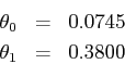
of gradient descent from this initial starting point. Record the value of
of
), and run one iteration
of gradient descent from this initial starting point. Record the value of
of ![]() and
and ![]() that you get after this first iteration. (To verify that
your implementation is correct, later we'll ask you to check your values of
that you get after this first iteration. (To verify that
your implementation is correct, later we'll ask you to check your values of ![]() and
and ![]() against ours.)
against ours.)
2. Continue running gradient descent for more iterations until ![]() converges.
(this will take a total of about 1500 iterations). After convergence, record the
final values of
converges.
(this will take a total of about 1500 iterations). After convergence, record the
final values of ![]() and
and ![]() that you get.
that you get.
When you have found ![]() , plot the
straight line fit from your algorithm on the same graph as your training data.
The plotting commands will look something like this:
, plot the
straight line fit from your algorithm on the same graph as your training data.
The plotting commands will look something like this:
hold on % Plot new data without clearing old plot
plot(x(:,2), x*theta, '-') % remember that x is now a matrix with 2 columns
                           % and the second column contains the time info
legend('Training data', 'Linear regression')
Note that for most machine learning problems, ![]() is very high dimensional, so we don't be
able to plot
is very high dimensional, so we don't be
able to plot ![]() . But since in this example we have only one feature, being able
to plot this gives a nice sanity-check on our result.
. But since in this example we have only one feature, being able
to plot this gives a nice sanity-check on our result.
3. Finally, we'd like to make some predictions using the learned hypothesis. Use your model to predict the height for a two boys of age 3.5 and age 7.
Debugging If you are using Matlab/Octave and seeing many errors at runtime, try inspecting your matrix operations to check that you are multiplying and adding matrices in ways that their dimensions would allow. Remember that Matlab/Octave by default interprets an operation as a matrix operation. In cases where you don't intend to use the matrix definition of an operator but your expression is ambiguous to Matlab/Octave, you will have to use the 'dot' operator to specify your command. Additionally, you can try printing x, y, and theta to make sure their dimensions are correct.
Understanding ![]()
We'd like to understand better what gradient descent has done, and visualize the relationship between
the parameters
![]() and
and ![]() . In this problem, we'll plot
. In this problem, we'll plot ![]() as a 3D surface plot.
(When applying learning algorithms, we don't usually try to plot
as a 3D surface plot.
(When applying learning algorithms, we don't usually try to plot ![]() since usually
since usually
![]() is
very high-dimensional so that we don't have any simple way to plot or visualize
is
very high-dimensional so that we don't have any simple way to plot or visualize ![]() . But because the
example here uses a very low dimensional
. But because the
example here uses a very low dimensional
![]() , we'll plot
, we'll plot ![]() to gain more intuition about
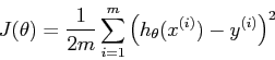
linear regression.) Recall that the formula for
to gain more intuition about
linear regression.) Recall that the formula for ![]() is
is
J_vals = zeros(100, 100);   % initialize Jvals to 100x100 matrix of 0's
theta0_vals = linspace(-3, 3, 100);
theta1_vals = linspace(-1, 1, 100);
for i = 1:length(theta0_vals)
	  for j = 1:length(theta1_vals)
	  t = [theta0_vals(i); theta1_vals(j)];
	  J_vals(i,j) = %% YOUR CODE HERE %%
    end
end

% Plot the surface plot
% Because of the way meshgrids work in the surf command, we need to
% transpose J_vals before calling surf, or else the axes will be flipped
J_vals = J_vals'
figure;
surf(theta0_vals, theta1_vals, J_vals)
xlabel('\theta_0'); ylabel('\theta_1')
You should get a figure similar to the following. If you are using Matlab/Octave, you can use the orbit tool to view this plot from different viewpoints.

What is the relationship between this 3D surface and the value of ![]() and
and ![]() that your implementation
of gradient descent had found?
that your implementation
of gradient descent had found?